Master Stability Function
Understanding Chaos: An Example
Imagine a hypothetical point particle in motion in 3D space. How would you find the trajectory of this hypothetical point particle? This would be very easy if you knew the equations of motion of the particle. But if you don’t have those, the next best thing to know is the velocity vector of this point particle at every point in space. From there you can obtain the equations of motion.
Lorenz system describes such a point particle in 3D space. Its velocity vectors are given by the following equations, $$ \begin{aligned} \dot{x}(t) &= \sigma(y - x) \\ \dot{y}(t) &= x(\rho - z) - y \\ \dot{z}(t) &= xy - \beta z \end{aligned} $$
with constants $\sigma, \rho ,$ and $\beta$. Usually we take $\sigma = 10$, $\rho = 28$ and $\beta = 8/3$.
The equations of motion for the Lorenz system would be the analytical solution to the differential equations above. However, this system does not possess an analytical solution that is known to us. Despite this, the trajectory can still be determined approximately using numerical methods.
Above shown is the projection of the solution of the Lorenz system in 3D space to the xz-plane with two different initial conditions, $(1,1,1)$ (red) and $(1.01,1.01,1.01)$ (white). Initially both particles seem to follow a similar path (we can’t see red as it’s covered by white) but after some time the paths are extremely different.
The difference in paths described above is known as chaotic behaviour. However, it’s important not to mistake this for predictability. Because we use numerical methods, the solutions we obtain are only approximations. The example demonstrates that these numerical solutions can approximate the actual solution accurately only for a limited period. Therefore, unpredictability in chaos implies that we cannot integrate numerically to determine the long-term behaviour of the system.
Coupled Dynamical System
We can combine multiple Lorenz system to get a new dynamical system in a higer dimensional space. For example we can couple two Lorenz system through x variable to get a system in 6D space.
Example
We can couple two Lorenz equations using the continuous functions $h_1,h_2,h_3,h_4 : \mathbb{R}^3 \to \mathbb{R}$
$$ \begin{aligned} \dot{x_1}(t) &= \sigma(y_1 - x_1) \color{red}{+ k \left[h_1(x_1,y_1,z_1)+h_2(x_2,y_2,z_2 )\right]} \\ \dot{y_1}(t) &= x_1(\rho - z_1) - y_1 \\ \dot{z_1}(t) &= x_1y_1 - \beta z_1 \\ \dot{x_2}(t) &= \sigma(y_2 - x_2) \color{red}{+ k \left[h_3(x_1,y_1,z_1)+h_4(x_2,y_2,z_2 )\right]} \\ \dot{y_2}(t) &= x_2(\rho - z_2) - y_2 \\ \dot{z_2}(t) &= x_2y_2 - \beta z_2 \end{aligned} $$ where k is the coupling constant and $ (x_1,y_1,z_1,x_2,y_2,z_2 ) \in \mathbb{R}^6$. We can think of this system as a two particles moving in $\mathbb{R}^3$ or as a single particle in $\mathbb{R}^{6}$.
Synchronisation Manifold
Thinking of solution of above example as the trajectory of a point particle sitting in $\mathbb{R}^6$. It’s position coordinate can take values like:
- $(0,1,2,2,1,3)$
- $(0.1,2,100,25.51,\pi,e)$
- $(0.24,3.15,5.12,0.24,3.15,5.12)$
What’s the speciality of the last one? For the last one $x_1=x_2,y_1=y_2,z_1=z_2 $, ie when thinking this example as two particle system in $\mathbb{R}^3$ their paths are overlapping. Under what conditions we can observe such a synchronised state from an experimental setup?
- The system should stay in the synchronised state for some amount of time. In other words after the sytem entered the synchronised state it should continue in synchronised state. Let’s use our brain, This situation is the same as both particles following the same path. So, if they have to follow the same path their velocities should match, ie, coupling terms (shown in red) in above equation should vanish.
- If the system is starting from a non-synchrchronous state, it should be able to enter the synchronised states.
We call the subset of $\mathbb{R}^6$ with all synchronised state the Synchronisation Manifold. Which is same as the set $$\{(x_1,y_1,z_1,x_2,y_2,z_2) \quad | \quad x_1=x_2, y_1=y_2, z_1=z_2 \}$$
Networks
A network is a system of interconnected entities or nodes that communicate, share resources, or collaborate to achieve common goals.
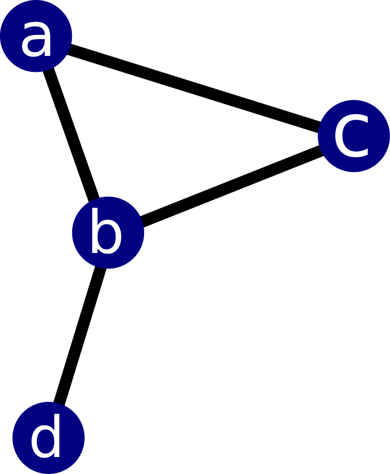
A network with 4 vertices and 4 links between them. The vertices are labelled as a,b,c,d
We can couple any number of dynamical systems to form a more extensive dynamical system in a higher dimension. We will get a network if we consider each dynamical system as the vertex/node and the coupling between them as the link/edge between the vertices. This network is an easy way to visualise our newly formed dynamic system. The topology of this underlying network is an essential factor in determining the stability of the coupled equation.
Laplacian matrix for this network will be a matrix with diagonals representing the degree of each vertex (the number of connections it has) and off-diagonal elements representing the connections between vertices. For the network shown in the image, the Laplacian matrix L would be:
$$ \begin{matrix} & a & b & c & d & \\ a & 2 & -1 & -1 & 0 \\ b & -1 & 3 & -1 & -1 \\ c & -1 & -1 & 2 & 0 \\ d & 0 & -1 & 0 & 1 \end{matrix} $$
Lyapunov exponents
Lyapunov exponents measure the average exponential rate of divergence or convergence of nearby trajectories in a dynamical system.

If $\lambda > 0$, nearby trajectories diverge exponentially, indicating chaos. If $\lambda < 0$, nearby trajectories converge exponentially, indicating stability. If $\lambda=0$ nearby trajectories stay close without converging or diverging.
Synchronisation
Suppose we have a network of $N$ identical dynamical system, and $\textbf{L}= (L_{ij})$ be the corresponding Laplacian matrix. Let $x_i \in \mathbb{R}^m$ and $f:\mathbb{R}^m\to\mathbb{R}^m$, if $\dot{x_i} = f(x_i)$ is the equation for a dynamical system then,
$$ \dot{x_i} = f(x_i) - k\sum_{j=1}^N L_{ij} h(x_j) $$ will be the equation for the whole network where, $k$ is the coupling constant and $h:\mathbb{R}^m\to\mathbb{R}^m$ is the coupling function. Note that the solution of this equation lives in $\mathbb{R}^{mN}$.
The synchronisation manifold is $m$-dimensional sub manifold of $\mathbb{R}^{mN}$ satisfying the condition: $$x_1 = x_2 = \ldots = x_{N-1} = x_N = x_s \qquad x_s \in R^m$$
Master Stability Function
If we define $\mu = -k \lambda$, where $\lambda$ is the eigenvalue of the Laplacian matrix L and k is the coupling constant.
$$ \dot{\eta} = \left[Df(x_s) + \mu Dh(x_s)\right]\eta $$
Now, we can define the master stability function $MSF(\mu)$ , for a particular dynamical system $\dot{x}=f(x)$, and the coupling function $h$, as the function that maps $\mu$ to the maximal Lyapunov exponent $\Lambda_{max}(\mu)$ of the above equation.
Interpreting the Master stability function
When the coupling constant equals zero, each node adheres to its own dynamic behaviour, characterized by chaos, and results in a positive maximum Lyapunov exponent. The master stability function of a coupled chaotic system can be broadly classified into three distinct categories.
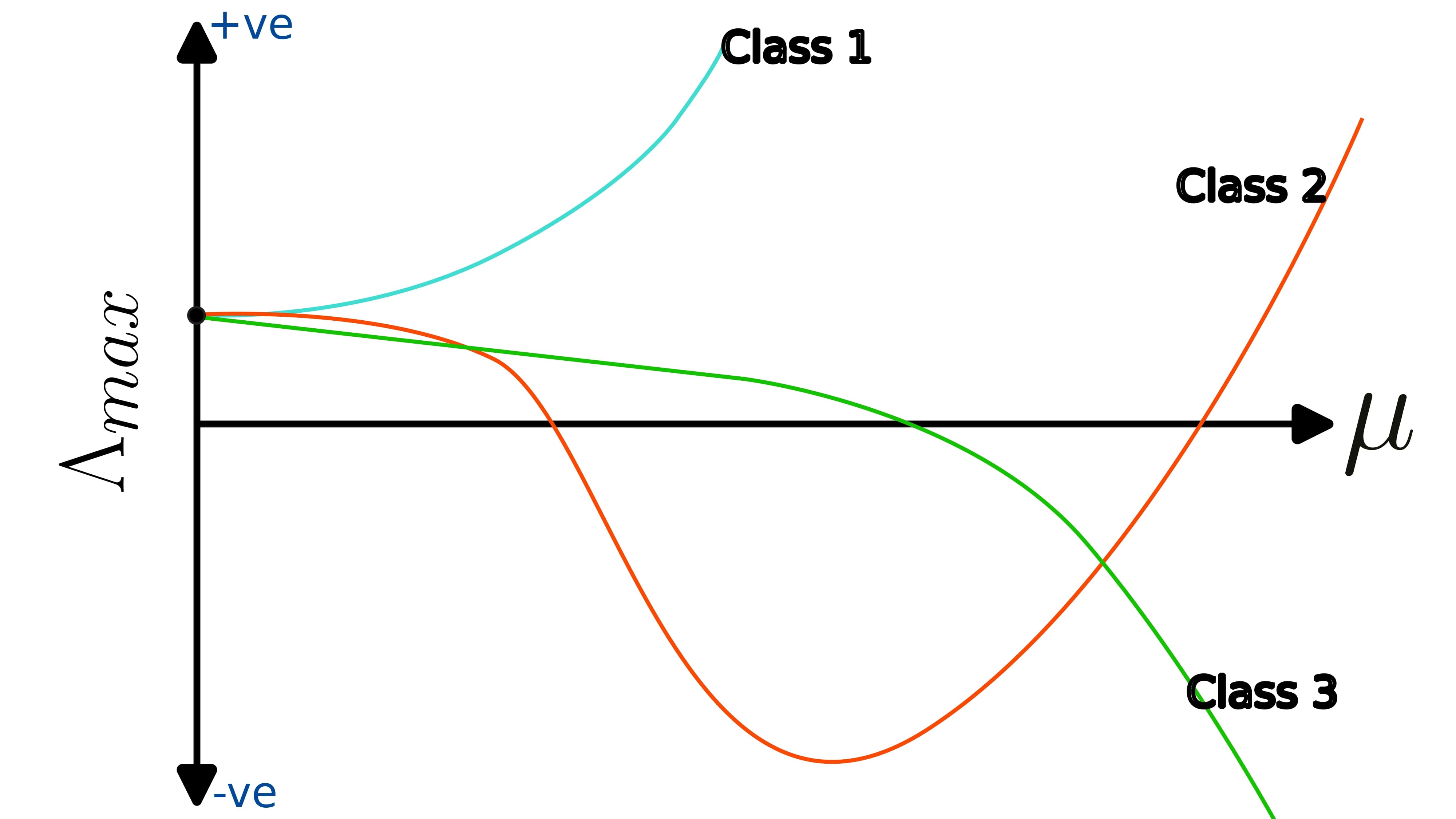
Class 1: $\Lambda_{max}>0$ when $\mu=0$ and the function stays positive when $\mu>0$. When master stability functions are of this type, the synchronisation manifold will not be a stable manifold for any kind of networks with positive coupling constant $\sigma$.
Class 2: $\Lambda_{max}>0$ when $\mu=0$ then the function becomes negative for some values of $0<\mu<\tilde{\mu}$ and again becomes positive when $\mu>\tilde{\mu}$. For dynamical system with class 2 master stability function, the synchronisation manifold will be stable only for some network topologies. Specifically the ones whose laplacian matrix’s eigen values are close to each other.
Class 3: $\Lambda_{max}>0$ when $\mu=0$ and function becomes negative for some values of $\mu$ and remains negative. The synchronisation manifold for dynamical systems with this type of master stability function will be stable for every kind of network topologies with sufficiently large coupling constant $\sigma$.
Note that when N is very large, say 1 billion, numerically solving is the coupled equation is a tedious job. But with the help of master stability function we can find the stability of synchronised stated by numerically integrating a much simpler equation.
References
Huang, L., Chen, Q., Lai, Y.-C., & Pecora, L. M. (2009). Generic behavior of master-stability functions in coupled nonlinear dynamical systems. Physical Review E, 80(3), 036204. https://link.aps.org/doi/10.1103/PhysRevE.80.036204
Pecora, L. M., & Carroll, T. L. (1998). Master Stability Functions for Synchronized Coupled Systems. Physical Review Letters, 80(10), 2109-2112. https://link.aps.org/doi/10.1103/PhysRevLett.80.2109
Strogatz, S. H. (2015). Nonlinear Dynamics and Chaos: With Applications to Physics, Biology, Chemistry, and Engineering (2nd ed.). CRC Press. https://doi.org/10.1201/9780429492563